Comparing Self-Esteem Across Ages with Moderated Nonlinear Factor Analysis
Introduction
A researcher plans to compare self-esteem between children aged 8 to 14. The 900 children come from a research panel of families, one child per family, with ages spread evenly. Age is computed from the date of birth. Each child completes a 10-item self-esteem questionnaire with five positively worded and five negatively worded items. Items are rated from 1, strongly disagree, to 5, strongly agree, and the negatively worded items are reverse-scored. The researcher is concerned that younger children respond differently to the negatively worded items.
Comparing total scores across ages assumes measurement invariance. The usual test compares item intercepts and loadings across groups, so age is cut into bands. Children within a band are then treated as the same age, and the result can change with the cut points. The researcher needs to know whether the intercepts and loadings of the negatively worded items change with age, without age bands.
Research Question
Should the five negatively worded items be included in the total score that the researcher uses to compare self-esteem between children aged 8 to 14?
Method
Bauer and Hussong (2009) and Bauer (2017) define moderated nonlinear factor analysis (MNLFA) as a factor model whose item parameters and factor distribution depend on observed covariates. The covariate is age, a continuous variable. The 900 children are all children aged 8 to 14 in the panel. The intercepts and loadings of the negatively worded items change linearly with age, so differential item functioning (DIF) across age is estimated without age bands. The factor mean and variance also change with age, which separates a change in self-esteem from a change in the items.
Model
For child $i$ and item $j$, the model is
\[y_{ij} = \nu_{0j} + \nu_{1j} a_i + \left(\lambda_{0j} + \lambda_{1j} a_i\right)\eta_i + \varepsilon_{ij}, \qquad \varepsilon_{ij} \sim N(0, \theta_j)\] \[\eta_i \sim N\!\left(\alpha_1 a_i,\ \exp(\beta_1 a_i)\right)\]where
- $y_{ij}$ is the score of child $i$ on item $j$, from 1 to 5,
- $a_i$ is the age of child $i$ minus 11 years,
- $\eta_i$ is the self-esteem of child $i$,
- $\nu_{0j}$ and $\lambda_{0j}$ are the intercept and loading of item $j$ at age 11,
- $\nu_{1j}$ and $\lambda_{1j}$ are the changes in the intercept and loading of item $j$ per year of age,
- $\theta_j$ is the residual variance of item $j$,
- $\alpha_1$ is the change in the factor mean per year of age,
- $\beta_1$ is the change in the log of the factor variance per year of age.
The factor mean is 0 and the factor variance is 1 at age 11, which sets the scale of $\eta_i$. The five positively worded items are anchor items, with $\nu_{1j}$ and $\lambda_{1j}$ fixed at 0. Without anchor items, a change in $\alpha_1$ cannot be distinguished from changes in all intercepts in proportion to the loadings. A positive $\nu_{1j}$ means that older children score higher on item $j$ than younger children with the same self-esteem. A positive $\lambda_{1j}$ means that the score on item $j$ is more strongly related to self-esteem in older children. The invariant model fixes $\nu_{1j}$ and $\lambda_{1j}$ at 0 for all 10 items, and the DIF model frees them for the five negatively worded items. Both models are estimated by maximum likelihood (ML).
Assumptions
- Unidimensionality: one factor, self-esteem, accounts for the covariances of the 10 items at every age, and the residuals are uncorrelated.
- Anchor items: the intercepts and loadings of the five positively worded items do not change with age.
- The intercepts, the loadings, the factor mean, and the log of the factor variance change linearly with age.
- Conditional normality: given $\eta_i$ and $a_i$, each item score, treated as continuous, is normally distributed with a residual variance that does not change with age.
Quantities of Interest
Age Moderation of the Negatively Worded Items
The estimates of $\nu_{1j}$ and $\lambda_{1j}$ in the DIF model measure the yearly change in the intercept and loading of each negatively worded item. They are reported with standard errors, Wald 95% confidence intervals, and Wald $z$ tests and do not enter the criterion.
Likelihood Ratio Statistic
\[LR = -2\ell_{\text{inv}} - \left(-2\ell_{\text{DIF}}\right)\]$\ell_{\text{inv}}$ and $\ell_{\text{DIF}}$ are the maximized log-likelihoods of the invariant and DIF models. $LR$ tests the 10 moderation parameters jointly. When the invariant model is true, $LR$ follows a $\chi^2$ distribution with 10 degrees of freedom in large samples.
The researcher sets the significance level at .05 before the analysis. The $p$ value of $LR$ is the probability of an $LR$ at least as large as the observed one when the invariant model is true. If it is below .05, the five negatively worded items are left out of the total score used to compare ages. If it is .05 or above, the 10-item total score is kept.
Analysis
The analysis uses five packages.
| Package | Purpose |
|---|---|
OpenMx | Fit and compare the invariant and DIF models |
dplyr | Summarize item scores and select parameter estimates |
tidyr | Reshape item scores and model-implied parameters |
knitr | Print the results table in Markdown |
ggplot2 | Plot model-implied intercepts and loadings by age |
1
2
3
4
5
6
7
8
9
10
11
12
13
14
15
16
17
18
19
# Setup ----
library(OpenMx)
library(tidyverse)
library(knitr)
N_CHILDREN <- 900
AGE_MIN <- 8
AGE_MAX <- 14
AGE_CENTER <- 11
ITEM_NAMES <- str_c("item", str_pad(1:10, width = 2, pad = "0"))
NEGATIVE_ITEMS <- ITEM_NAMES[6:10]
FACTOR_MEAN_SLOPE <- 0.03
FACTOR_LOGVAR_SLOPE <- 0
ITEM_LOADING <- rep(c(0.75, 0.60), each = 5)
ITEM_LOADING_SLOPE <- rep(c(0, 0.05), each = 5)
ITEM_INTERCEPT_SLOPE <- rep(c(0, 0.05), each = 5)
THRESHOLDS <- c(-1.8, -1.1, -0.3, 0.5)
DIF_LABELS <- c(str_c("nu1_", NEGATIVE_ITEMS), str_c("lambda1_", NEGATIVE_ITEMS))
theme_portfolio <- theme_minimal(base_size = 13) +
  theme(panel.grid.minor = element_blank(), legend.position = "bottom")
Simulate Survey Responses
The data are simulated to match the scenario, with 900 children, their age in years, and scores from 1 to 5 on 10 items. The columns item01 to item05 hold the positively worded items, and item06 to item10 the reverse-scored negatively worded items.
1
2
3
4
5
6
7
8
9
10
11
12
13
14
15
16
17
18
19
20
21
22
23
24
25
26
27
28
29
30
31
# Simulate Survey Responses ----
set.seed(1124)
age <- round(runif(N_CHILDREN, min = AGE_MIN, max = AGE_MAX), 1)
age_c <- age - AGE_CENTER
self_esteem <- rnorm(N_CHILDREN, mean = FACTOR_MEAN_SLOPE * age_c, sd = sqrt(exp(FACTOR_LOGVAR_SLOPE * age_c)))
responses <- pmap(
  list(ITEM_LOADING, ITEM_LOADING_SLOPE, ITEM_INTERCEPT_SLOPE),
  \(lambda0, lambda1, nu1) {
    latent_response <- nu1 * age_c + (lambda0 + lambda1 * age_c) * self_esteem +
      rnorm(N_CHILDREN, mean = 0, sd = sqrt(1 - lambda0^2))
    findInterval(latent_response, THRESHOLDS) + 1L
  }
) %>%
  set_names(ITEM_NAMES) %>%
  as_tibble() %>%
  mutate(age = age, .before = 1)
print(responses)
#> # A tibble: 900 × 11
#>      age item01 item02 item03 item04 item05 item06 item07 item08 item09 item10
#>    <dbl>  <int>  <int>  <int>  <int>  <int>  <int>  <int>  <int>  <int>  <int>
#>  1  11.7      1      2      5      3      3      4      4      1      4      4
#>  2   8.6      5      4      5      5      5      5      3      3      4      5
#>  3   8.3      5      5      5      5      5      5      5      5      4      5
#>  4   8.5      1      3      2      1      1      3      3      3      3      5
#>  5   8.4      4      3      4      5      5      3      4      5      5      4
#>  6  13.4      5      5      4      4      5      5      4      5      5      5
#>  7  11        4      4      3      3      2      3      4      4      3      4
#>  8   9.9      4      4      4      3      3      5      4      5      4      5
#>  9  13.1      2      3      3      1      4      3      5      3      5      2
#> 10  11.7      5      5      5      4      5      4      5      4      4      3
#> # ℹ 890 more rows
Describe Item Scores
summarise() computes the sample size n and the mean, standard deviation, minimum, and maximum of age. For each item, it computes the mean, the standard deviation, and r_age, the Pearson correlation with age. cor() prints the Pearson correlations among the 10 items.
1
2
3
4
5
6
7
8
9
10
11
12
13
14
15
16
17
18
19
20
21
22
23
24
25
26
27
28
29
30
31
32
33
34
35
36
37
38
# Describe Item Scores ----
age_summary <- responses %>%
  summarise(n = n(), mean_age = mean(age), sd_age = sd(age), min_age = min(age), max_age = max(age))
item_summary <- responses %>%
  pivot_longer(all_of(ITEM_NAMES), names_to = "item", values_to = "score") %>%
  group_by(item) %>%
  summarise(mean = mean(score), sd = sd(score), r_age = cor(score, age), .groups = "drop")
print(age_summary)
#> # A tibble: 1 × 5
#>       n mean_age sd_age min_age max_age
#>   <int>    <dbl>  <dbl>   <dbl>   <dbl>
#> 1   900     11.0   1.73       8      14
print(item_summary)
#> # A tibble: 10 × 4
#>    item    mean    sd   r_age
#>    <chr>  <dbl> <dbl>   <dbl>
#>  1 item01  3.82  1.08 0.00682
#>  2 item02  3.77  1.11 0.0277
#>  3 item03  3.82  1.06 0.00610
#>  4 item04  3.79  1.05 0.0347
#>  5 item05  3.81  1.08 0.0274
#>  6 item06  3.83  1.08 0.0816
#>  7 item07  3.83  1.06 0.0302
#>  8 item08  3.81  1.06 0.0516
#>  9 item09  3.85  1.06 0.0544
#> 10 item10  3.84  1.09 0.0554
print(round(cor(responses[ITEM_NAMES]), 2))
#>        item01 item02 item03 item04 item05 item06 item07 item08 item09 item10
#> item01   1.00   0.51   0.50   0.51   0.47   0.41   0.36   0.34   0.36   0.42
#> item02   0.51   1.00   0.52   0.50   0.48   0.42   0.36   0.35   0.36   0.38
#> item03   0.50   0.52   1.00   0.50   0.50   0.39   0.39   0.32   0.36   0.36
#> item04   0.51   0.50   0.50   1.00   0.51   0.41   0.35   0.33   0.36   0.40
#> item05   0.47   0.48   0.50   0.51   1.00   0.39   0.38   0.35   0.36   0.36
#> item06   0.41   0.42   0.39   0.41   0.39   1.00   0.29   0.30   0.31   0.30
#> item07   0.36   0.36   0.39   0.35   0.38   0.29   1.00   0.32   0.26   0.27
#> item08   0.34   0.35   0.32   0.33   0.35   0.30   0.32   1.00   0.25   0.27
#> item09   0.36   0.36   0.36   0.36   0.36   0.31   0.26   0.25   1.00   0.24
#> item10   0.42   0.38   0.36   0.40   0.36   0.30   0.27   0.27   0.24   1.00
The 900 children had a mean age of 11.0 years ($SD$ = 1.73), from 8 to 14. Item means ranged from 3.77 for item02 to 3.85 for item09, and standard deviations from 1.05 for item04 to 1.11 for item02. r_age ranged from 0.00610 to 0.0347 for the positively worded items and from 0.0302 to 0.0816 for the negatively worded items. The item correlations ranged from 0.24, item09 with item10, to 0.52, item02 with item03.
Fit the Invariant Model
mxModel() specifies the model in matrices, with L0, L1, N0, N1, and Theta for the item parameters and A1 and B1 for $\alpha_1$ and $\beta_1$. The label data.age_c sets Age to each child’s age_c, and mxAlgebra() builds each child’s model-implied mean Mu and covariance Sigma. L1 and N1 are fixed at 0 with free = FALSE, and mxRun() fits the model by ML. For alpha1 and beta1, the script prints the estimate, the standard error, the Wald 95% confidence limits ci_lower and ci_upper, the Wald z statistic, and its two-sided p value.
1
2
3
4
5
6
7
8
9
10
11
12
13
14
15
16
17
18
19
20
21
22
23
24
25
26
27
28
29
30
31
32
# Fit the Invariant Model ----
mnlfa_data <- responses %>%
  mutate(age_c = age - AGE_CENTER) %>%
  as.data.frame()
mnlfa_invariant <- mxModel(
  "invariant",
  mxData(mnlfa_data, type = "raw"),
  mxMatrix("Full", nrow = 10, ncol = 1, free = TRUE, values = 0.8, labels = str_c("lambda0_", ITEM_NAMES), name = "L0"),
  mxMatrix("Full", nrow = 10, ncol = 1, free = FALSE, values = 0, labels = str_c("lambda1_", ITEM_NAMES), name = "L1"),
  mxMatrix("Full", nrow = 1, ncol = 10, free = TRUE, values = 3.7, labels = str_c("nu0_", ITEM_NAMES), name = "N0"),
  mxMatrix("Full", nrow = 1, ncol = 10, free = FALSE, values = 0, labels = str_c("nu1_", ITEM_NAMES), name = "N1"),
  mxMatrix("Diag", nrow = 10, ncol = 10, free = TRUE, values = 0.5, labels = str_c("theta_", ITEM_NAMES), name = "Theta"),
  mxMatrix("Full", nrow = 1, ncol = 1, free = TRUE, values = 0, labels = "alpha1", name = "A1"),
  mxMatrix("Full", nrow = 1, ncol = 1, free = TRUE, values = 0, labels = "beta1", name = "B1"),
  mxMatrix("Full", nrow = 1, ncol = 1, free = FALSE, labels = "data.age_c", name = "Age"),
  mxAlgebra(L0 + L1 %x% Age, name = "L"),
  mxAlgebra(N0 + N1 %x% Age, name = "N"),
  mxAlgebra(A1 %x% Age, name = "Alpha"),
  mxAlgebra(exp(B1 %x% Age), name = "Psi"),
  mxAlgebra(L %*% Psi %*% t(L) + Theta, name = "Sigma"),
  mxAlgebra(N + t(L %*% Alpha), name = "Mu"),
  mxExpectationNormal(covariance = "Sigma", means = "Mu", dimnames = ITEM_NAMES),
  mxFitFunctionML()
)
fit_invariant <- mxRun(mnlfa_invariant)
#> Running invariant with 32 parameters
print(fit_invariant$output$status$code)
#> [1] 0
print(summary(fit_invariant)$parameters %>% filter(name %in% c("alpha1", "beta1")) %>% transmute(name, Estimate, Std.Error, ci_lower = Estimate - qnorm(0.975) * Std.Error, ci_upper = Estimate + qnorm(0.975) * Std.Error, z = Estimate / Std.Error, p = 2 * pnorm(-abs(z))))
#>     name   Estimate  Std.Error     ci_lower   ci_upper        z          p
#> 1 alpha1 0.03169998 0.02070357 -0.008878280 0.07227823 1.531136 0.12573589
#> 2  beta1 0.06924627 0.03059403  0.009283075 0.12920946 2.263392 0.02361156
The invariant model had 32 free parameters. Its status code was 0, which OpenMx returns for a successful optimization. The estimates were $\alpha_1$ = 0.032 ($SE$ = 0.021, 95% $CI$ = [-0.009, 0.072], $p$ = 0.126) and $\beta_1$ = 0.069 ($SE$ = 0.031, 95% $CI$ = [0.009, 0.129], $p$ = 0.024).
Fit the Model with Age-Moderated Items
omxSetParameters() frees the 10 parameters in DIF_LABELS, the entries of N1 and L1 for item06 to item10, with free = TRUE and name = "dif". The script prints the status code and, for these parameters, alpha1, and beta1, the same six columns as in the invariant model.
1
2
3
4
5
6
7
8
9
10
11
12
13
14
15
16
17
18
19
20
# Fit the Model with Age-Moderated Items ----
mnlfa_dif <- omxSetParameters(mnlfa_invariant, labels = DIF_LABELS, free = TRUE, name = "dif")
fit_dif <- mxRun(mnlfa_dif)
#> Running dif with 42 parameters
print(fit_dif$output$status$code)
#> [1] 0
print(summary(fit_dif)$parameters %>% filter(name %in% c(DIF_LABELS, "alpha1", "beta1")) %>% transmute(name, Estimate, Std.Error, ci_lower = Estimate - qnorm(0.975) * Std.Error, ci_upper = Estimate + qnorm(0.975) * Std.Error, z = Estimate / Std.Error, p = 2 * pnorm(-abs(z))))
#>              name   Estimate  Std.Error     ci_lower   ci_upper         z          p
#> 1  lambda1_item06 0.02196203 0.01848514 -0.014268176 0.05819223 1.1880911 0.23479751
#> 2  lambda1_item07 0.04555646 0.01883698  0.008636652 0.08247628 2.4184584 0.01558643
#> 3  lambda1_item08 0.04209357 0.01886496  0.005118915 0.07906822 2.2313091 0.02566066
#> 4  lambda1_item09 0.01567731 0.01874213 -0.021056583 0.05241121 0.8364746 0.40288798
#> 5  lambda1_item10 0.03995708 0.01897510  0.002766562 0.07714759 2.1057636 0.03522490
#> 6      nu1_item06 0.04112778 0.01782772  0.006186094 0.07606946 2.3069570 0.02105722
#> 7      nu1_item07 0.01072662 0.01810328 -0.024755167 0.04620840 0.5925233 0.55350022
#> 8      nu1_item08 0.02424855 0.01832094 -0.011659844 0.06015694 1.3235424 0.18565507
#> 9      nu1_item09 0.02480973 0.01826576 -0.010990510 0.06060996 1.3582640 0.17437994
#> 10     nu1_item10 0.02623906 0.01832355 -0.009674434 0.06215256 1.4319858 0.15214789
#> 11         alpha1 0.01851927 0.02114725 -0.022928582 0.05996713 0.8757295 0.38117712
#> 12          beta1 0.03707943 0.03183335 -0.025312795 0.09947166 1.1647981 0.24410071
The DIF model had 42 free parameters and status code 0. The estimates of $\lambda_{1j}$ ranged from 0.016 for item09 to 0.046 for item07, and those of $\nu_{1j}$ from 0.011 for item07 to 0.041 for item06. All 10 estimates were positive, and their standard errors ranged from 0.018 to 0.019. Four of the 10 estimates had $p$ below 0.05, the $\lambda_{1j}$ of item07, item08, and item10 and the $\nu_{1j}$ of item06. In this model, $\alpha_1$ = 0.019 ($SE$ = 0.021, 95% $CI$ = [-0.023, 0.060], $p$ = 0.381) and $\beta_1$ = 0.037 ($SE$ = 0.032, 95% $CI$ = [-0.025, 0.099], $p$ = 0.244).
Test Age Moderation of the Negatively Worded Items
mxCompare() computes the likelihood ratio test of the invariant model against the DIF model. For each model, it reports the number of estimated parameters ep, minus2LL, the degrees of freedom df, and AIC. diffLL is the difference in minus2LL, which is $LR$, with degrees of freedom diffdf and $p$ value p.
1
2
3
4
5
# Test Age Moderation of the Negatively Worded Items ----
print(mxCompare(fit_dif, fit_invariant))
#>   base comparison ep minus2LL   df      AIC   diffLL diffdf          p
#> 1  dif       <NA> 42 24046.38 8958 24130.38       NA     NA         NA
#> 2  dif  invariant 32 24069.22 8968 24133.22 22.84226     10 0.01134404
minus2LL was 24046.38 for the DIF model and 24069.22 for the invariant model. diffLL was 22.84 on diffdf = 10, with p = 0.011. df, the number of observed statistics minus ep, was 8958 and 8968, and AIC was 24130.38 and 24133.22.
Build the Table and Figure
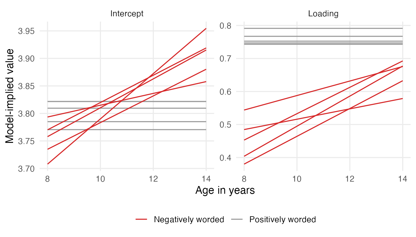
The script collects the 10 moderation parameters with their standard errors, confidence intervals, and Wald $z$ tests into a table printed by kable(). It also plots the model-implied intercepts and loadings of the DIF model from age 8 to 14.
1
2
3
4
5
6
7
8
9
10
11
12
13
14
15
16
17
18
19
20
21
22
23
24
25
26
27
28
29
30
31
32
33
34
35
36
37
38
39
40
41
# Build the Table and Figure ----
results_table <- summary(fit_dif)$parameters %>%
  filter(name %in% DIF_LABELS) %>%
  as_tibble() %>%
  transmute(
    parameter = str_c(if_else(str_detect(name, "^nu1"), "Intercept", "Loading"), ", Item ", as.integer(str_extract(name, "\\d+$"))),
    estimate = Estimate,
    se = Std.Error,
    ci_lower = Estimate - qnorm(0.975) * Std.Error,
    ci_upper = Estimate + qnorm(0.975) * Std.Error,
    z = Estimate / Std.Error,
    p = 2 * pnorm(-abs(z))
  )
print(kable(
  results_table,
  format = "pipe",
  digits = 3,
  col.names = c("Parameter", "Estimate", "SE", "95% CI lower", "95% CI upper", "z", "p")
))
implied_parameters <- tibble(
  item = ITEM_NAMES,
  lambda0 = as.vector(fit_dif$L0$values),
  lambda1 = as.vector(fit_dif$L1$values),
  nu0 = as.vector(fit_dif$N0$values),
  nu1 = as.vector(fit_dif$N1$values)
) %>%
  crossing(age = seq(AGE_MIN, AGE_MAX, by = 0.1)) %>%
  mutate(
    Loading = lambda0 + lambda1 * (age - AGE_CENTER),
    Intercept = nu0 + nu1 * (age - AGE_CENTER),
    wording = if_else(item %in% NEGATIVE_ITEMS, "Negatively worded", "Positively worded")
  ) %>%
  pivot_longer(c(Intercept, Loading), names_to = "parameter", values_to = "value")
figure1 <- implied_parameters %>%
  ggplot(aes(x = age, y = value, group = item, colour = wording)) +
  geom_line() +
  facet_wrap(~ parameter, scales = "free_y") +
  scale_colour_manual(values = c(`Negatively worded` = "#D62728", `Positively worded` = "grey60")) +
  labs(x = "Age in years", y = "Model-implied value", colour = NULL) +
  theme_portfolio
ggsave("output/figure1.png", figure1, width = 7, height = 4, dpi = 200)
The output of this step is Table 1 and Figure 1 in Results.
Results
MNLFA was fitted to the 10 item scores of 900 children aged 8 to 14 ($M$ = 11.0, $SD$ = 1.73). There were no missing data. Item means ranged from 3.77 to 3.85, and item correlations from .24 to .52. The invariant and DIF models, with 32 and 42 free parameters, converged normally. To test whether the intercepts and loadings of the five negatively worded items varied with age, the two models were compared with a likelihood ratio test. The test rejected the invariant model in favor of the DIF model, $\chi^2$(10) = 22.84, $p$ = .011.
In the DIF model, all 10 age moderation estimates were positive (Table 1). The intercept estimates $\hat\nu_{1j}$ ranged from 0.011 to 0.041 points per year of age, and the loading estimates $\hat\lambda_{1j}$ ranged from 0.016 to 0.046 per year (Figure 1). Four estimates were significant at the .05 level, the loadings of Items 7, 8, and 10 and the intercept of Item 6. The age slope of the factor mean was not significant in either model, $\hat{\alpha}_1$ = 0.032 ($SE$ = 0.021, 95% $CI$ = [-0.009, 0.072], $p$ = .126) in the invariant model and 0.019 ($SE$ = 0.021, 95% $CI$ = [-0.023, 0.060], $p$ = .381) in the DIF model.
Table 1. Age moderation of the intercepts and loadings of the five negatively worded items in the DIF model
| Parameter | Estimate | SE | 95% CI lower | 95% CI upper | z | p |
|---|---|---|---|---|---|---|
| Loading, Item 6 | 0.022 | 0.018 | -0.014 | 0.058 | 1.188 | 0.235 |
| Loading, Item 7 | 0.046 | 0.019 | 0.009 | 0.082 | 2.418 | 0.016 |
| Loading, Item 8 | 0.042 | 0.019 | 0.005 | 0.079 | 2.231 | 0.026 |
| Loading, Item 9 | 0.016 | 0.019 | -0.021 | 0.052 | 0.836 | 0.403 |
| Loading, Item 10 | 0.040 | 0.019 | 0.003 | 0.077 | 2.106 | 0.035 |
| Intercept, Item 6 | 0.041 | 0.018 | 0.006 | 0.076 | 2.307 | 0.021 |
| Intercept, Item 7 | 0.011 | 0.018 | -0.025 | 0.046 | 0.593 | 0.554 |
| Intercept, Item 8 | 0.024 | 0.018 | -0.012 | 0.060 | 1.324 | 0.186 |
| Intercept, Item 9 | 0.025 | 0.018 | -0.011 | 0.061 | 1.358 | 0.174 |
| Intercept, Item 10 | 0.026 | 0.018 | -0.010 | 0.062 | 1.432 | 0.152 |
Figure 1. Model-implied intercepts and loadings of the 10 items from age 8 to 14 in the DIF model
Discussion
MNLFA was used to examine whether the intercepts and loadings of the five negatively worded self-esteem items varied with age between 8 and 14, and the likelihood ratio test rejected their invariance, $p$ = .011. Following the prespecified criterion, the five negatively worded items were excluded from the total score used to compare self-esteem across ages.
The joint test and the four significant estimates are consistent with the concern that younger children respond differently to negatively worded items. The loadings of Items 7, 8, and 10 increased with age, which indicates that scores on these items were more strongly related to self-esteem in older children. The intercept of Item 6 increased by 0.041 points per year, so older children scored higher on this item than younger children with the same self-esteem. The other six estimates were positive but not significant. A total score that includes items with age-dependent intercepts mixes an age difference in self-esteem with an age difference in item functioning. The age slope of the factor mean was not significant in either model, so the data do not establish an age trend in self-esteem. Under the model, a total score of the five positively worded items has the same relation to self-esteem at every age from 8 to 14.
Limitations
This conclusion rests on the invariance of the five positively worded items across age. If an anchor item changes with age, the model attributes part of that change to $\alpha_1$ and $\beta_1$, and the estimates of $\nu_{1j}$ and $\lambda_{1j}$ shift in the opposite direction. The item scores are treated as continuous, which attenuates the loadings and weakens the $\chi^2$ approximation of $LR$. The linear age terms describe children aged 8 to 14 and do not extend to younger or older children.