Shortening a Vocabulary Placement Test

Background

Vocabulary-learning products need an initial estimate of a learner’s ability to recommend content at an appropriate difficulty. The placement test that produces this estimate is part of onboarding. A longer assessment improves precision, and it also increases the effort required before users receive any value from the product.

This trade-off matters more when users with different linguistic backgrounds take the same English assessment. A vocabulary item can be easy or difficult for reasons other than the ability the test intends to measure.

Product Question

Can the placement test be shortened without weakening placement decisions for both native and non-native English speakers?

Data

Vocabulary IQ Test (VIQT)

The test consists of 45 vocabulary items. Each item asks the respondent to identify a pair of words with the same meaning. The dataset includes responses from 12,173 respondents, along with item-level response times and demographic information including native-English status. The data are publicly available from the Open Source Psychometrics Project.

Analysis Sample

• Respondents with a reported age outside 13-100 years excluded
• Respondents without a native or non-native classification excluded

After these restrictions, the analysis sample contained 12,103 respondents, with 9,366 native English speakers and 2,737 non-native English speakers.

Variables Used

• Item responses
• Item response time
• Native-English status

Problem Definition

Three problems arise when all 45 items are used for placement.

Efficiency

The full test requires about 6.9 minutes, based on the sum of item-level median response times.

Placement happens before personalization begins. Every additional question therefore adds onboarding cost, and long tests can cause users to leave the product.

Measurement Quality

Not every item contributes equally to scoring and classification.

Some items may have low discrimination, meaning they do not separate learners with different levels of vocabulary ability.

Others may be too easy or too difficult to provide information around the boundaries where classification decisions change.

Group Comparability

Some items may function differently by native-English status.

If two respondents have the same underlying ability but different probabilities of answering an item correctly because of language background, that item is undesirable for a common placement test.

Objective

Build a shorter test that maximizes Fisher information at the placement boundaries within a time budget, exclude items that function differently by native-English status, and measure how closely the short form reproduces the full-test scores and placement levels.

Methods

The analysis was conducted in R using four main packages.

Package	Purpose
mirt	Estimate item parameters, item information, and respondent ability
lordif	Identify items that function differently for native and non-native speakers
TestDesign	Select the most informative set of items within the time budget
ggplot2	Visualize item selection and short-form performance

Estimate Item Characteristics and Ability

Item response theory (IRT) places items and respondents on one ability scale, so each item can be evaluated by how much information it contributes at a given ability level. A two-parameter logistic (2PL) model was fitted to the 45 binary-scored items using mirt.

For item $i$,

\[P_i(\theta) = \frac{1} {1+\exp[-a_i(\theta-b_i)]}\]

where

• $a_i$ is item discrimination,
• $b_i$ is item difficulty,
• $\theta$ is vocabulary ability.

From the 2PL response function, item information is given by

\[I_i(\theta)=a_i^2P_i(\theta)\left[1-P_i(\theta)\right].\]

Item information measures precision at a given ability level. $b_i$ determines where information is concentrated, and $a_i$ determines its magnitude.

IRT scoring weights each response by the item’s parameters. Two respondents with the same number of correct answers receive different estimates when they answered different items correctly. Respondent ability was estimated by expected a posteriori (EAP) estimation in mirt,

\[\hat{\theta}_{EAP} = E(\theta \mid \mathbf{u}),\]

where $\mathbf{u}$ denotes the respondent’s item-response pattern.

Define the Classification Decision

The cut points were set at $\theta$ = -1 and $\theta$ = 1, one standard deviation below and above the mean of the ability scale. They define three placement levels.

• Level 1: $\theta$ ≤ -1
• Level 2: -1 < $\theta$ ≤ 1
• Level 3: $\theta$ > 1

Thus,

\[c_1=-1,\qquad c_2=1.\]

These values are the two boundaries where the classification decision changes.

Screen Items for Differential Item Functioning

Differential item functioning (DIF) analysis identifies items with different response probabilities for native and non-native speakers at the same estimated vocabulary ability.

DIF was examined by native-English status using lordif, which uses an iterative hybrid of IRT and logistic regression. It models each item response as a function of estimated ability and measures the change in pseudo $R^2$ when group membership is added.

DIF detection used

• criterion = "R2"
• pseudo.R2 = "McFadden"

with the package’s default $R^2$-change threshold of .02.

Items flagged for DIF were excluded from the candidate item pool before test assembly.

Optimize the Test for a 3-Minute Time Budget

A 3-minute budget was set to cut the 6.9-minute testing time by more than half. Classification is most sensitive to estimation error near the two cut points, so the short form was assembled to maximize information at these boundaries.

The target estimated testing time was

\[T=180\text{ seconds}.\]

For each item $i$,

• $x_i$ = 1 if the item is selected and 0 otherwise,
• $t_i$ is the item’s median response time,
• $I_i(c_1)$ and $I_i(c_2)$ are its information values at the two cut points.

Because item information is additive, the test information for a selected set of items at ability $\theta$ is

\[I_T(\theta) = \sum_i x_i I_i(\theta).\]

The assembly objective was to maximize information at the two cut points

\[\max \sum_i x_i \left[ \frac{I_i(c_1)+I_i(c_2)}{2} \right]\]

subject to the time constraint

\[\sum_i t_i x_i \le 180\]

and

\[x_i=0 \quad \text{for DIF-flagged items}.\]

The two cut points received equal weight because crossing either boundary changes the assigned level. Optimization was performed with TestDesign using the MAXINFO criterion.

Fixed-form assembly requires a specified test length. Every feasible length was assembled under the same 180-second constraint, and the form with the greatest cut-point information was retained.

Evaluation Metrics

The following metrics measure what the short form preserves and what it loses.

Estimated Test Time

\[T_{\text{short}} = \sum_{i \in S} t_i\]

where $S$ is the selected set of items. The sum of item-level median response times estimates the typical duration of the test.

Quadratic Weighted Kappa (QWK)

\[\kappa_w = 1- \frac{\sum_{r,s} w_{rs}O_{rs}} {\sum_{r,s} w_{rs}E_{rs}}, \qquad w_{rs}= \left(\frac{r-s}{K-1}\right)^2\]

QWK measures agreement between ordered placement levels. It corrects for chance agreement and weights a disagreement by the squared distance between the two levels.

Root Mean Square Difference (RMSD)

\[\text{RMSD} = \sqrt{ \frac{1}{N} \sum_{j=1}^{N} \left( \hat\theta_j^{\text{short}} - \hat\theta_j^{\text{full}} \right)^2 }\]

RMSD measures how much the short-form ability estimates deviate from the full-test estimates.

Results

Measurement Quality

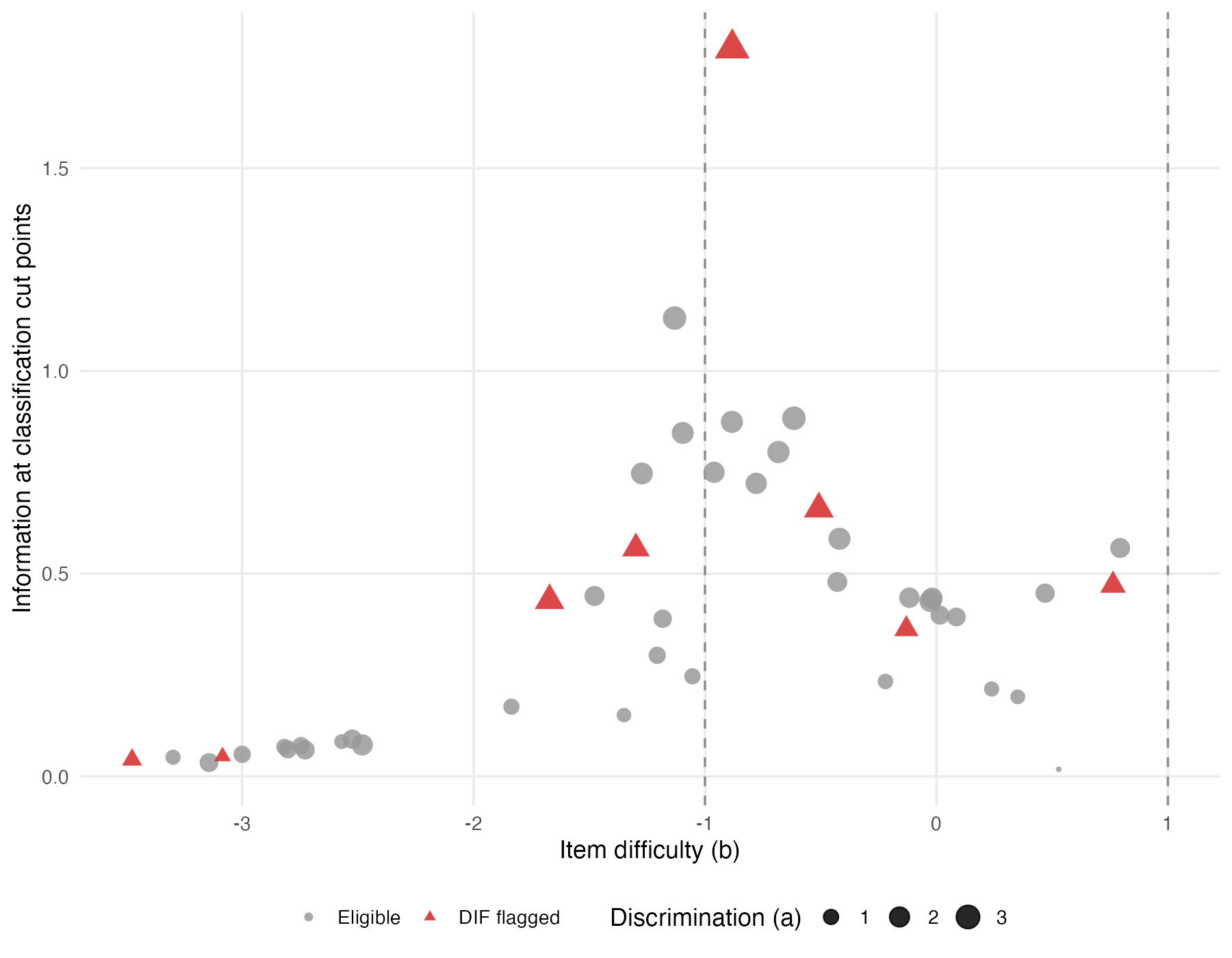
As shown in the figure, every item had a difficulty parameter below the upper cut point at $\theta$ = 1. Of the 45 items, 37 had a negative difficulty parameter, and the largest estimate was $b$ = 0.79.

Twelve items had $b$ below -2. They were pairs of common words, such as large and big (Q1, $b$ = -3.14, 98.2% correct), rob and steal (Q3, $b$ = -2.73, 97.3% correct), and drop and fall (Q16, $b$ = -3.30, 95.3% correct). Each of the twelve had a mean information across the two cut points below 0.10.

Eight items had a positive $b$. The two most difficult pairs were fractious and querulous (Q43, $b$ = 0.79, 26.8% correct) and incipient and nascent (Q27, $b$ = 0.76, 28.6% correct). The lowest discrimination belonged to deal and sale (Q7, $a$ = 0.27), with a mean cut-point information of 0.02.

Information in the 2PL model peaks at $\theta$ = $b_i$. Sixteen items had $b$ within 0.5 of the lower cut point, and three items had $b$ within 0.5 of the upper cut point. The item pool therefore supports the boundary between Level 1 and Level 2 with more items than the boundary between Level 2 and Level 3.

Group Comparability

lordif flagged 8 of 45 items for DIF by native-English status.

Item	Synonym pair	Correct	$a$	$b$	Pseudo $R^2$ change
Q17	fly, soar	92.3%	2.63	-1.67	0.1059
Q24	lackluster, drab	80.0%	3.88	-0.88	0.0617
Q27	incipient, nascent	28.6%	1.86	0.76	0.0481
Q33	house, domicile	85.3%	2.21	-1.30	0.0299
Q36	epistle, letter	53.9%	1.62	-0.13	0.0277
Q10	partner, companion	95.6%	1.02	-3.48	0.0273
Q39	yearn, hanker	67.2%	2.68	-0.51	0.0271
Q26	annoying, obnoxious	87.5%	0.69	-3.08	0.0240

The flagged items covered the difficulty range of the pool, from partner and companion ($b$ = -3.48) to incipient and nascent ($b$ = 0.76). Fly and soar had the largest pseudo $R^2$ change at 0.1059, more than five times the .02 threshold. The other seven items ranged from 0.0240 to 0.0617.

The exclusion removed items that the assembly would otherwise rank highly. Lackluster and drab had the highest discrimination ($a$ = 3.88) and the largest mean cut-point information (1.80) of the 45 items. Incipient and nascent was one of the three items with $b$ within 0.5 of the upper cut point. After the exclusion, the candidate pool contained 37 items, with 13 items within 0.5 of the lower cut point and two within 0.5 of the upper cut point.

Optimized 3-Minute Test

TestDesign selected 19 items with an estimated testing time of 2.95 minutes against the 3.0-minute budget. Compared with the 6.9-minute full test, this is a 57.1% reduction in estimated testing time.

The selected items had $b$ from -1.48 to 0.79 and $a$ from 1.46 to 3.08. Sixteen had a negative $b$, and three had a positive $b$: bifurcate and fork (Q40), stanchion and pole (Q38), and fractious and querulous (Q43). Of the 18 eligible items left out, 11 had $b$ below -1.8 and six had $a$ below 1.26. The remaining item, muster and convene (Q18, $a$ = 1.82, $b$ = 0.02), had the longest median response time of the 45 items at 14.4 seconds.

The short form provided more information at the lower cut point ($I$ = 19.09 at $\theta$ = -1) than at the upper cut point ($I$ = 4.26 at $\theta$ = 1). Placement between Level 2 and Level 3 is therefore less precise than placement between Level 1 and Level 2.

Scoring and Classification Performance

	45-item test	Optimized short form
Items	45	19
Estimated time	6.9 min	3.0 min
Time reduction	—	57.1%
QWK	Reference	0.848
RMSD	—	0.242

The short form had a QWK of 0.848 against the full-test placement levels and an RMSD of 0.242 against the full-test ability estimates. A QWK of 0.848 is within the 0.81-1.00 range that Landis and Koch (1977) label almost perfect agreement. An RMSD of 0.242 is about a quarter of a standard deviation on the $\theta$ scale, against a distance of two standard deviations between the cut points.

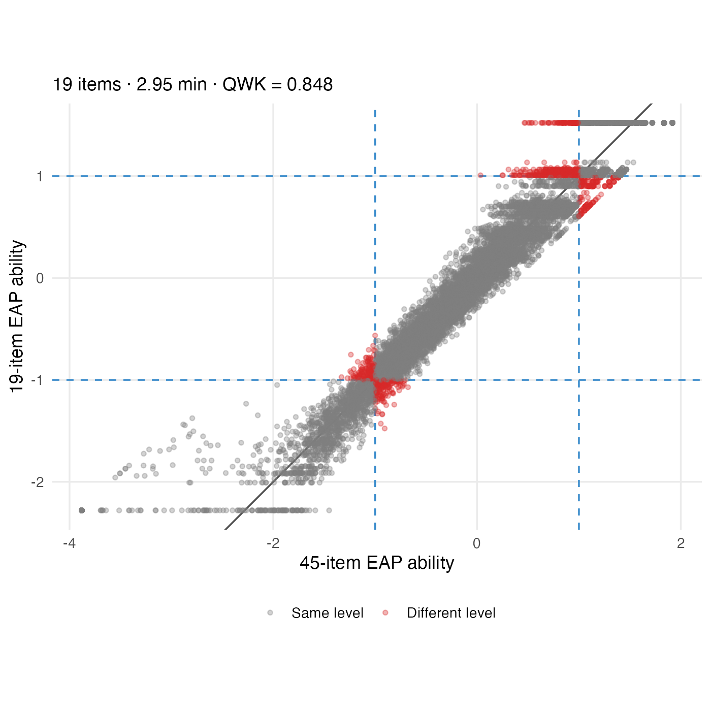
As shown in the figure, respondents whose placement level changed were concentrated around the two cut points, where a small difference in estimated ability moves a respondent into an adjacent level. A level change under the short form therefore affects learners whose full-test estimate is already close to a boundary.

Recommendation

Strengthen measurement for higher-ability learners

Of the 45 items, 37 had a negative difficulty parameter, and no item had $b$ above 0.79. The short form provided $I$ = 4.26 at $\theta$ = 1 against $I$ = 19.09 at $\theta$ = -1. New items with $b$ near 1 would raise precision at the upper cut point.

Remove the 8 DIF-flagged items

The eight flagged items exceeded the .02 pseudo $R^2$ change threshold, led by fly and soar at 0.1059 and lackluster and drab at 0.0617. Remove or revise these items before deploying the short form.

Use 19 items for a 3-minute placement test

Nineteen items, selected to maximize information at the cut points, reduced estimated testing time by 57.1%. The short form reproduced full-test placement levels with a QWK of 0.848, within the 0.81-1.00 range labeled almost perfect agreement.

Limitation

DIF was screened by native-English status and not by age. An item that functions differently across the 13-100 age range is not excluded on that basis, and the agreement metrics, which compare the short form with the full test, do not detect it.

Code

library(mirt)
library(lordif)
library(TestDesign)
library(tidyverse)

raw <- read.delim("VIQT_data.csv", sep = "\t")

ITEM_COLS <- str_c("Q", 1:45)
TIME_COLS <- str_c("E", 1:45)
TARGET_SEC <- 180
CUTS <- c(-1, 1)

ANSWER_KEY <- c(
  24,3,10,5,9,9,17,10,17,10,5,17,9,5,18,18,3,12,18,18,
  3,18,6,12,17,10,10,9,9,3,6,10,17,3,17,24,17,5,5,24,
  5,5,12,10,9
)

classify <- function(x, cuts) cut(x, c(-Inf, cuts, Inf), labels = FALSE)

raw <- raw %>% filter(engnat %in% 1:2, between(age, 13, 100))

X <- (as.matrix(raw[ITEM_COLS]) == matrix(ANSWER_KEY, nrow(raw), 45, byrow = TRUE)) * 1L
colnames(X) <- ITEM_COLS
grp <- as.integer(raw$engnat == 2)

item_sec <- raw[TIME_COLS] %>% map_dbl(~ median(.x, na.rm = TRUE) / 1000) %>% set_names(ITEM_COLS)
total_sec <- sum(item_sec)

mod <- mirt(X, 1, itemtype = "2PL", verbose = FALSE)
pars <- coef(mod, IRTpars = TRUE, simplify = TRUE)$items
theta_full <- fscores(mod, method = "EAP")[, 1]
class_full <- classify(theta_full, CUTS)

dif <- lordif(as.data.frame(X + 1), grp, criterion = "R2", pseudo.R2 = "McFadden")
dif_flag <- as.logical(dif$flag)
r2_dif <- as.numeric(dif$stats$pseudo13.McFadden)

pool <- loadItemPool(mod)[which(!dif_flag)]
attrib <- loadItemAttrib(data.frame(ID = pool@id, TIME = item_sec[pool@id]), pool)
config <- createStaticTestConfig(
  item_selection = list(method = "MAXINFO", info_type = "FISHER", target_location = CUTS, target_weight = c(1, 1)),
  MIP = list(solver = "lpSolve", verbosity = -2)
)
max_k <- sum(cumsum(sort(item_sec[!dif_flag])) <= TARGET_SEC)

assemble_k <- function(k) {
  spec <- data.frame(CONSTRAINT_ID = c("LENGTH", "TIME"), 
                     TYPE = c("Number", "Sum"), 
                     WHAT = "Item", 
                     CONDITION = c("", "TIME"), 
                     LB = c(k, 0), 
                     UB = c(k, TARGET_SEC), 
                     ONOFF = "")
  solution <- Static(config, loadConstraints(spec, pool, attrib))
  tibble(k = k, objective = solution@obj_value, items = list(pool@id[solution@selected$INDEX]), solution = list(solution))
}

assemblies <- map(seq_len(max_k), assemble_k) %>% list_rbind()
best <- assemblies %>% slice_max(objective, n = 1, with_ties = FALSE)
selected <- best$items[[1]]
selected_k <- best$k
solution <- best$solution[[1]]
short_sec <- sum(item_sec[selected])

X_short <- X
X_short[, !ITEM_COLS %in% selected] <- NA
theta_short <- fscores(mod, method = "EAP", response.pattern = X_short)[, 1]
class_short <- classify(theta_short, CUTS)

obs <- table(factor(class_full, 1:3), factor(class_short, 1:3))
expected <- outer(rowSums(obs), colSums(obs)) / sum(obs)
w <- outer(1:3, 1:3, function(r, s) ((r - s) / 2)^2)
kappa <- 1 - sum(w * obs) / sum(w * expected)
rmsd <- sqrt(mean((theta_short - theta_full)^2))
info_cut <- map_dbl(1:45, ~ mean(iteminfo(extract.item(mod, .x), matrix(CUTS))))

card <- tibble(
  item = ITEM_COLS,
  pct_correct = colMeans(X),
  median_sec = item_sec,
  a = pars[, "a"],
  b = pars[, "b"],
  info_cut = info_cut,
  r2_dif = r2_dif,
  dif_flag = dif_flag,
  selected = ITEM_COLS %in% selected
) %>%
  mutate(
    status = case_when(selected ~ "Selected", dif_flag ~ "DIF flagged", TRUE ~ "Not selected"),
    screen_status = if_else(dif_flag, "DIF flagged", "Eligible")
  )

assembly_result <- assemblies %>% transmute(n_items = k, objective, minutes = map_dbl(items, ~ sum(item_sec[.x]) / 60))

summary_result <- tibble(
  respondents = nrow(X),
  full_items = 45,
  selected_items = selected_k,
  target_minutes = TARGET_SEC / 60,
  estimated_minutes = short_sec / 60,
  full_minutes = total_sec / 60,
  time_saved_pct = 100 * (1 - short_sec / total_sec),
  quadratic_weighted_kappa = kappa,
  rmsd = rmsd,
  dif_flagged_items = sum(dif_flag)
)

write_csv(card, "output/item_selection.csv")
write_csv(assembly_result, "output/testdesign_candidates.csv")
write_csv(summary_result, "output/summary.csv")


theme_portfolio <- theme_minimal(base_size = 13) + theme(panel.grid.minor = element_blank(), legend.position = "bottom")

p1 <- ggplot(card, aes(b, info_cut)) +
  geom_vline(xintercept = CUTS, linetype = 2, color = "grey55") +
  geom_point(aes(size = a, color = screen_status, shape = screen_status), alpha = .85) +
  scale_color_manual(values = c("Eligible" = "grey60", "DIF flagged" = "#D62728")) +
  scale_shape_manual(values = c("Eligible" = 16, "DIF flagged" = 17)) +
  labs(x = "Item difficulty (b)", y = "Information at classification cut points", size = "Discrimination (a)", color = NULL, shape = NULL) +
  theme_portfolio
ggsave("output/figure1.png", p1, width = 9, height = 7, dpi = 200)

theta_plot <- tibble(full = theta_full, short = theta_short, classification = if_else(class_short == class_full, "Same level", "Different level"))

p2 <- ggplot(theta_plot, aes(full, short)) +
  geom_vline(xintercept = CUTS, linetype = 2, color = "#3C8DCC") +
  geom_hline(yintercept = CUTS, linetype = 2, color = "#3C8DCC") +
  geom_abline(color = "grey30") +
  geom_point(aes(color = classification), alpha = .35, size = 1.2) +
  scale_color_manual(values = c("Same level" = "grey50", "Different level" = "#D62728")) +
  coord_equal() +
  labs(x = "45-item EAP ability", y = str_c(selected_k, "-item EAP ability"), color = NULL) +
  theme_portfolio
ggsave("output/figure2.png", p2, width = 7, height = 7, dpi = 200)


print(summary_result, width = Inf)
card %>% filter(selected) %>% select(item, median_sec, a, b, info_cut, r2_dif) %>% print(n = Inf)
print(assembly_result, n = Inf)
summary(solution)