Timing Support in a Wellbeing App

Background

Wellbeing apps ask users to rate how they feel several times a day. The app uses the answers to decide when to offer a short exercise, a prompt, or a suggestion to contact someone. These decisions are part of the product experience, and a poorly timed prompt interrupts a user who no longer needs it.

A single rating shows the level at one moment. It does not show how long that level lasts or what follows it. Deciding when to respond requires knowing how ratings change from one check-in to the next.

Product Question

Should the app respond to a single elevated check-in, and does the same rule fit every user?

Data

COVID-19 Student ESM Study

Fried et al. (2022) followed 80 undergraduate students in the Netherlands for 14 days in March 2020. Students answered a short questionnaire four times a day, giving up to 56 check-ins per person. The data are publicly available through the openESM database (dataset 0001).

Analysis Sample

• Participants with fewer than 20 complete check-ins excluded

After this restriction, the analysis sample contained 75 participants and 3,883 check-ins, 92.5% of their scheduled prompts.

Variables Used

• Worry, rated 1 (not at all) to 5 (extremely)
• Alone, feeling a lack of companionship, rated on the same scale
• Day and check-in number within day

Problem Definition

Three things are unknown when a single check-in is used as a trigger.

Persistence

A rating shows the level at one moment, not how much of it remains a few hours later.

If little remains, the feeling has usually passed by the time a second reading confirms it. If much remains, one reading is a strong signal and waiting costs little.

Ordering

Worry and loneliness are rated at the same time, so their order in time is not visible in the raw ratings.

If loneliness precedes worry, a loneliness report is an early cue worth acting on. If worry comes first, loneliness is a consequence and not a cue.

Heterogeneity

A rule tuned to the average user may not fit individual users.

The size of between-person differences decides whether one rule is enough or whether the app needs person-specific thresholds.

Objective

Estimate the carryover of worry and loneliness between check-ins, estimate the cross-lagged effects between them, separate the average effects from between-person differences, and convert the estimates into a rule for when the app responds.

Methods

The analysis was conducted in R using three main packages.

Package	Purpose
openesm	Download the harmonized experience sampling data
brms	Fit the dynamic structural equation model and compare models
ggplot2	Visualize person-specific effects and between-person differences

Model Check-in Dynamics with DSEM

A dynamic structural equation model (DSEM) treats each person’s check-ins as a short time series and treats the people as a sample from a population. It separates a person’s usual level from the way momentary deviations carry over from one check-in to the next.

For person $i$ at check-in $t$, worry follows

\[W_{it} = \mu^W_i + \phi^{WW}_i (W_{i,t-1}-\mu^W_i) + \phi^{WA}_i (A_{i,t-1}-\mu^A_i) + \beta^W \text{day}_t + e^W_{it}\]

and loneliness follows

\[A_{it} = \mu^A_i + \phi^{AA}_i (A_{i,t-1}-\mu^A_i) + \phi^{AW}_i (W_{i,t-1}-\mu^W_i) + \beta^A \text{day}_t + e^A_{it}\]

where

• $\mu^W_i$ and $\mu^A_i$ are person $i$’s usual levels,
• $\phi^{WW}_i$ and $\phi^{AA}_i$ are carryover effects,
• $\phi^{WA}_i$ and $\phi^{AW}_i$ are cross-lagged effects,
• $\beta^W$ and $\beta^A$ are linear trends across the 14 days,
• $e^W_{it}$ and $e^A_{it}$ are residuals, correlated within a check-in.

The person-specific quantities vary across people,

\[(\mu^W_i, \mu^A_i, \phi^{WW}_i, \phi^{WA}_i, \phi^{AA}_i, \phi^{AW}_i) \sim \mathcal{N}(\boldsymbol{\gamma}, \boldsymbol{\Sigma}).\]

$\boldsymbol{\gamma}$ describes the average user. The standard deviations in $\boldsymbol{\Sigma}$ describe how much users differ, and its correlations describe whether usual level and dynamics are related.

Lagged predictors were centered on each person’s mean, so carryover and cross-lagged effects describe within-person change. Consecutive check-ins within the same day were paired, giving 2,747 lagged pairs. The model was fitted in brms with four chains of 4,000 iterations and weakly informative priors.

Compare Models With and Without Cross-Lagged Effects

A model without cross-lagged effects was fitted to the same data. Leave-one-out cross-validation (LOO) compared the two models on the difference in expected log predictive density (elpd) and its standard error.

Derived Quantities

The estimates were converted into three quantities that map onto the product question.

Half-Life

\[h = \frac{\log 0.5}{\log \phi}\]

The number of check-ins needed for a deviation to shrink by half, given carryover $\phi$.

Standardized Cross-Lagged Effect

\[\phi^{WA}_{std} = \phi^{WA} \frac{s_A}{s_W}\]

where $s_A$ and $s_W$ are within-person standard deviations. This puts both directions on the same scale.

Share of Users Whose Interval Excludes Zero

\[\text{Share} = \frac{1}{N}\sum_{i=1}^{N} \mathbb{1}\left[\text{lower}_i > 0\right]\]

The proportion of users whose person-specific 95% interval lies above zero.

Results

Persistence

The intraclass correlation was 0.39 for worry and 0.56 for loneliness. About 61% of the variance in worry was within-person change around each user’s usual level, which a single survey does not measure.

Carryover was positive for both variables, $\phi^{WW}$ = 0.246 (95% $CI$ = [0.196, 0.296]) for worry and $\phi^{AA}$ = 0.266 (95% $CI$ = [0.190, 0.340]) for loneliness. About a quarter of a worry deviation remained at the next check-in and about 6% two check-ins later. The half-life was 0.50 check-ins (95% $CI$ = [0.43, 0.57]). Three quarters of a worry deviation was gone by the next check-in a few hours later.

Worry also declined by 0.012 points per day, about 0.15 points across the two weeks.

Ordering

	Carryover only	DSEM with cross-lags
Loneliness to worry	Not included	0.117 (95% $CI$ = [0.041, 0.189])
Worry to loneliness	Not included	0.034 (95% $CI$ = [0.000, 0.068])
Standardized, to worry	Not included	0.084
Standardized, to loneliness	Not included	0.048
LOO difference (elpd)	Reference	+16.9 ($SE$ = 10.7)

A one-point rise in loneliness above a user’s usual level predicted a 0.12-point rise in worry at the next check-in, with a posterior probability of 0.998 that the effect was positive. The reverse path was 0.034 (95% $CI$ = [0.000, 0.068]). The difference in elpd between the model with cross-lagged effects and the model without was 16.9 ($SE$ = 10.7). For the app, a loneliness report predicts higher worry at the next check-in.

Heterogeneity

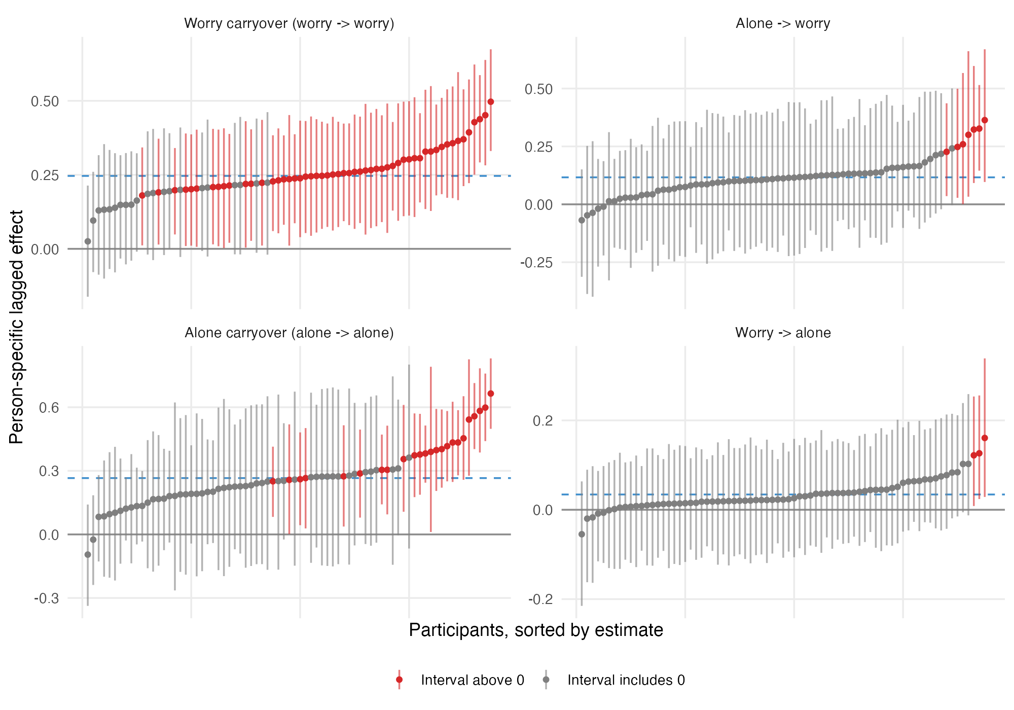
As shown in the figure, person-specific intervals for worry carryover lay above zero for most users, and intervals for the loneliness-to-worry effect included zero for most users.

Worry carryover ranged from 0.03 to 0.50 across users, and the person-specific 95% interval lay above zero for 54 of 75 users. For the loneliness-to-worry effect, the standard deviation across users (0.154) exceeded the average effect (0.117). Person-specific estimates ranged from -0.07 to 0.36, and the interval lay above zero for 7 of 75 users.

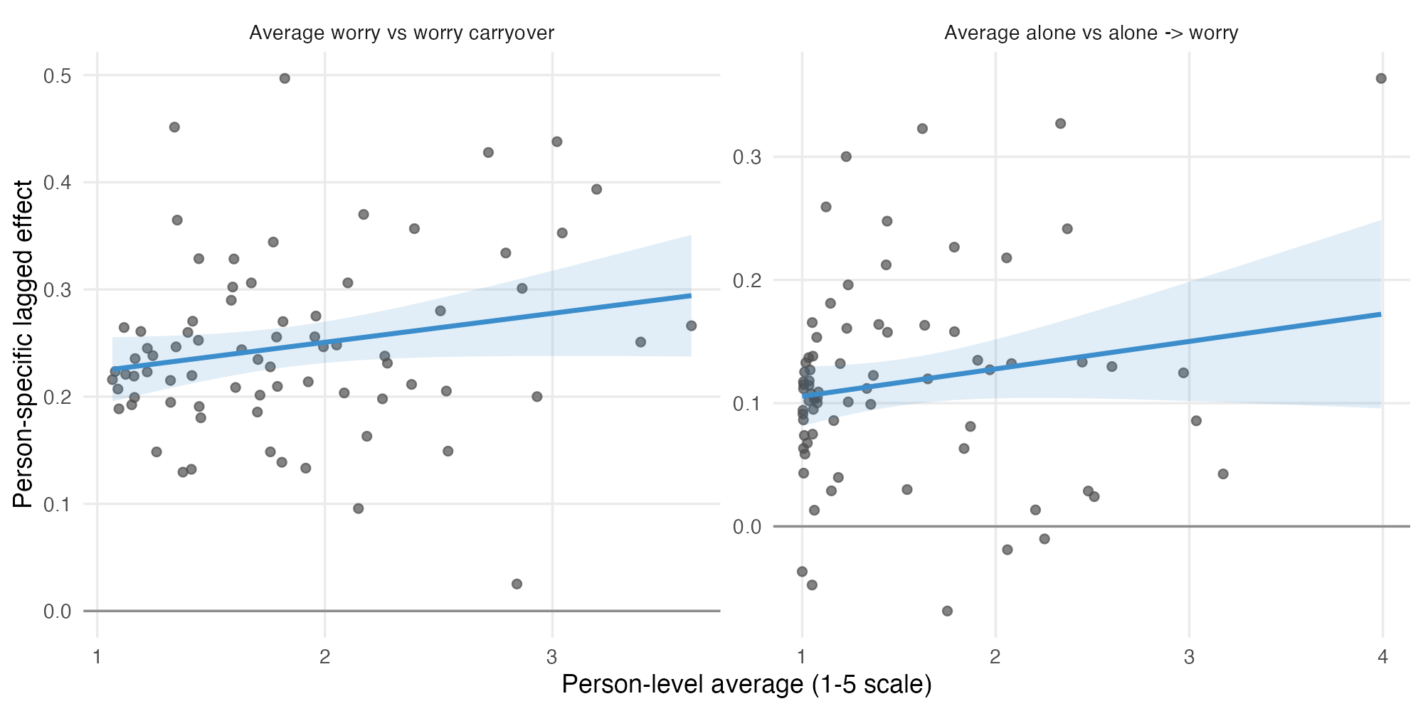
As shown in the figure, the correlations between usual level and person-specific effects had intervals that included zero. Users with higher average worry also had higher average loneliness ($r$ = 0.55, 95% $CI$ = [0.37, 0.69]). The correlation between average worry and worry carryover was 0.15 (95% $CI$ = [-0.20, 0.47]), and the correlation between average loneliness and the loneliness-to-worry effect was 0.03 (95% $CI$ = [-0.35, 0.40]).

Recommendation

Respond at the first elevated check-in

Three quarters of a worry deviation is gone by the next check-in, and the half-life is 0.50 check-ins. Waiting for a second reading means most episodes will have passed. The response should be light, because a quarter of the deviation remains at the next check-in.

Treat loneliness as a leading signal

A one-point rise in loneliness predicted a 0.12-point rise in worry at the next check-in, and the reverse path was 0.034 with a lower interval bound of 0.000. A loneliness report is a cue for social suggestions before worry rises.

Keep one rule until users have more data

After two weeks, the person-specific interval for the loneliness-to-worry effect lay above zero for 7 of 75 users. The correlations between usual level and dynamics had intervals that included zero. Person-specific thresholds should wait until several weeks of check-ins are available.

Limitation

Lagged predictors were centered on observed person means, which biases carryover estimates downward in short series. Lagged pairs were formed within days, so the estimates describe dynamics over a few hours and not overnight.

Code

library(openesm)
library(brms)
library(tidyverse)

ds <- get_dataset("0001")
raw <- ds$data %>% rename_with(tolower)

raw <- raw %>%
  transmute(id = as.character(id), day = as.integer(day), beep = as.integer(beep), worry = as.numeric(worry), alone = as.numeric(alone)) %>%
  drop_na(day, beep) %>%
  distinct(id, day, beep, .keep_all = TRUE)

n_day <- max(raw$day)
n_beep <- max(raw$beep)

d <- raw %>%
  complete(id, day = 1:n_day, beep = 1:n_beep) %>%
  arrange(id, day, beep) %>%
  group_by(id, day) %>%
  mutate(worry_lag = lag(worry), alone_lag = lag(alone)) %>%
  group_by(id) %>%
  mutate(n_obs = sum(!is.na(worry) & !is.na(alone))) %>%
  filter(n_obs >= 20) %>%
  mutate(
    worry_pm = mean(worry, na.rm = TRUE),
    alone_pm = mean(alone, na.rm = TRUE),
    worry_lag_c = worry_lag - worry_pm,
    alone_lag_c = alone_lag - alone_pm,
    day_c = day - mean(1:n_day)
  ) %>%
  ungroup()

obs_all <- d %>% drop_na(worry, alone)
md <- d %>% drop_na(worry, alone, worry_lag_c, alone_lag_c) %>% mutate(id = factor(id))

icc <- obs_all %>%
  group_by(id) %>%
  summarise(across(c(worry, alone), list(mean = mean, var = var))) %>%
  summarise(
    worry = var(worry_mean) / (var(worry_mean) + mean(worry_var, na.rm = TRUE)),
    alone = var(alone_mean) / (var(alone_mean) + mean(alone_var, na.rm = TRUE))
  )

descriptives <- tibble(
  variable = c("worry", "alone"),
  mean = c(mean(obs_all$worry), mean(obs_all$alone)),
  sd_total = c(sd(obs_all$worry), sd(obs_all$alone)),
  sd_within = c(sd(obs_all$worry - obs_all$worry_pm), sd(obs_all$alone - obs_all$alone_pm)),
  icc = c(icc$worry, icc$alone)
)

sample_summary <- tibble(
  participants_raw = n_distinct(raw$id),
  participants_kept = n_distinct(d$id),
  observations_kept = nrow(obs_all),
  lagged_pairs = nrow(md),
  possible_per_person = n_day * n_beep,
  compliance = nrow(obs_all) / (n_distinct(d$id) * n_day * n_beep),
  median_obs_per_person = median(distinct(d, id, n_obs)$n_obs)
)

priors <- c(
  prior(normal(2, 1.5), class = "Intercept", resp = "worry"),
  prior(normal(2, 1.5), class = "Intercept", resp = "alone"),
  prior(normal(0, 1), class = "b", resp = "worry"),
  prior(normal(0, 1), class = "b", resp = "alone"),
  prior(exponential(1), class = "sd", resp = "worry"),
  prior(exponential(1), class = "sd", resp = "alone"),
  prior(exponential(1), class = "sigma", resp = "worry"),
  prior(exponential(1), class = "sigma", resp = "alone"),
  prior(lkj(2), class = "cor"),
  prior(lkj(2), class = "rescor")
)

fit <- brm(
  bf(worry ~ 1 + day_c + worry_lag_c + alone_lag_c + (1 + worry_lag_c + alone_lag_c | p | id)) +
  bf(alone ~ 1 + day_c + worry_lag_c + alone_lag_c + (1 + worry_lag_c + alone_lag_c | p | id)) +
  set_rescor(TRUE),
  data = md, prior = priors,
  chains = 4, iter = 4000, warmup = 1000, cores = 4, seed = 20260910,
  control = list(adapt_delta = 0.95, max_treedepth = 12), refresh = 500
)
saveRDS(fit, "output/dsem_fit.rds")

fit0 <- brm(
  bf(worry ~ 1 + day_c + worry_lag_c + (1 + worry_lag_c | p | id)) +
  bf(alone ~ 1 + day_c + alone_lag_c + (1 + alone_lag_c | p | id)) +
  set_rescor(TRUE),
  data = md, prior = priors,
  chains = 4, iter = 4000, warmup = 1000, cores = 4, seed = 20260910,
  control = list(adapt_delta = 0.95, max_treedepth = 12), refresh = 500
)
saveRDS(fit0, "output/dsem_fit_no_crosslag.rds")

loo_table <- loo_compare(loo(fit), loo(fit0)) %>% as.data.frame() %>% rownames_to_column("model")

draws <- as_draws_df(fit)

fe <- fixef(fit) %>% as.data.frame() %>% rownames_to_column("term") %>%
  mutate(p_positive = map_dbl(term, ~ mean(draws[[paste0("b_", .x)]] > 0)))

vc <- VarCorr(fit)
re_sd <- vc$id$sd %>% as.data.frame() %>% rownames_to_column("term")

re_cor <- vc$id$cor %>% { list(estimate = .[, "Estimate", ], lower = .[, "Q2.5", ], upper = .[, "Q97.5", ]) } %>%
  map(~ as.data.frame(.x) %>% rownames_to_column("term_1") %>% pivot_longer(-term_1, names_to = "term_2")) %>%
  reduce(left_join, by = c("term_1", "term_2")) %>%
  set_names(c("term_1", "term_2", "estimate", "lower", "upper")) %>%
  filter(match(term_1, unique(term_1)) < match(term_2, unique(term_1)))

residual_cor <- tibble(
  estimate = median(draws$rescor__worry__alone),
  lower = quantile(draws$rescor__worry__alone, .025),
  upper = quantile(draws$rescor__worry__alone, .975)
)

half_life <- function(phi) log(0.5) / log(phi[phi > 0 & phi < 1])
hl_worry <- half_life(draws$b_worry_worry_lag_c)
hl_alone <- half_life(draws$b_alone_alone_lag_c)

half_life_summary <- tibble(
  variable = c("worry", "alone"),
  ar_median = c(median(draws$b_worry_worry_lag_c), median(draws$b_alone_alone_lag_c)),
  half_life_beeps = c(median(hl_worry), median(hl_alone)),
  half_life_lower = c(quantile(hl_worry, .025), quantile(hl_alone, .025)),
  half_life_upper = c(quantile(hl_worry, .975), quantile(hl_alone, .975))
)

sd_w <- deframe(descriptives[, c("variable", "sd_within")])
est <- deframe(fe[, c("term", "Estimate")])

std_effects <- tibble(
  path = c("worry -> worry", "alone -> worry", "alone -> alone", "worry -> alone"),
  raw = est[c("worry_worry_lag_c", "worry_alone_lag_c", "alone_alone_lag_c", "alone_worry_lag_c")],
  standardized = raw * c(1, sd_w["alone"] / sd_w["worry"], 1, sd_w["worry"] / sd_w["alone"])
)

cf <- coef(fit)$id
person_terms <- c("worry_Intercept", "worry_worry_lag_c", "worry_alone_lag_c", "alone_Intercept", "alone_alone_lag_c", "alone_worry_lag_c")

person <- map(person_terms, ~ tibble(id = dimnames(cf)[[1]], term = .x, estimate = cf[, "Estimate", .x], lower = cf[, "Q2.5", .x], upper = cf[, "Q97.5", .x])) %>% list_rbind()

person_wide <- person %>%
  select(id, term, estimate) %>%
  pivot_wider(names_from = term, values_from = estimate) %>%
  left_join(distinct(d, id, n_obs), by = "id")

heterogeneity <- person %>%
  filter(term %in% c("worry_worry_lag_c", "worry_alone_lag_c", "alone_alone_lag_c", "alone_worry_lag_c")) %>%
  group_by(term) %>%
  summarise(
    person_min = min(estimate),
    person_q25 = quantile(estimate, .25),
    person_median = median(estimate),
    person_q75 = quantile(estimate, .75),
    person_max = max(estimate),
    share_above_0.30 = mean(estimate > 0.30),
    share_interval_above_0 = mean(lower > 0),
    share_interval_below_0 = mean(upper < 0)
  )

write_csv(sample_summary, "output/sample_summary.csv")
write_csv(descriptives, "output/descriptives.csv")
write_csv(fe, "output/fixed_effects.csv")
write_csv(re_sd, "output/random_effect_sd.csv")
write_csv(re_cor, "output/random_effect_cor.csv")
write_csv(residual_cor, "output/residual_cor.csv")
write_csv(half_life_summary, "output/half_life.csv")
write_csv(std_effects, "output/standardized_effects.csv")
write_csv(person_wide, "output/person_effects.csv")
write_csv(heterogeneity, "output/heterogeneity.csv")
write_csv(loo_table, "output/model_comparison.csv")

theme_portfolio <- theme_minimal(base_size = 13) + theme(panel.grid.minor = element_blank(), legend.position = "bottom")

term_labels <- c(
  worry_worry_lag_c = "Worry carryover (worry -> worry)",
  worry_alone_lag_c = "Alone -> worry",
  alone_alone_lag_c = "Alone carryover (alone -> alone)",
  alone_worry_lag_c = "Worry -> alone"
)

plot_person <- person %>%
  filter(term %in% names(term_labels)) %>%
  mutate(
    label = factor(term_labels[term], levels = term_labels),
    sign = case_when(lower > 0 ~ "Interval above 0", upper < 0 ~ "Interval below 0", TRUE ~ "Interval includes 0")
  ) %>%
  group_by(label) %>%
  arrange(estimate, .by_group = TRUE) %>%
  mutate(rank = row_number()) %>%
  ungroup()

fe_lines <- tibble(label = factor(term_labels, levels = term_labels), estimate = est[names(term_labels)])

p1 <- ggplot(plot_person, aes(rank, estimate)) +
  geom_hline(yintercept = 0, color = "grey55") +
  geom_hline(data = fe_lines, aes(yintercept = estimate), linetype = 2, color = "#3C8DCC") +
  geom_linerange(aes(ymin = lower, ymax = upper, color = sign), alpha = .6) +
  geom_point(aes(color = sign), size = 1.4) +
  scale_color_manual(values = c("Interval above 0" = "#D62728", "Interval includes 0" = "grey50", "Interval below 0" = "#2C7BB6")) +
  facet_wrap(~ label, scales = "free_y") +
  labs(x = "Participants, sorted by estimate", y = "Person-specific lagged effect", color = NULL) +
  theme_portfolio +
  theme(axis.text.x = element_blank())
ggsave("output/figure1.png", p1, width = 10, height = 7, dpi = 200)

scatter <- bind_rows(
  tibble(x = person_wide$worry_Intercept, y = person_wide$worry_worry_lag_c, panel = "Average worry vs worry carryover"),
  tibble(x = person_wide$alone_Intercept, y = person_wide$worry_alone_lag_c, panel = "Average alone vs alone -> worry")
) %>% mutate(panel = fct_inorder(panel))

p2 <- ggplot(scatter, aes(x, y)) +
  geom_hline(yintercept = 0, color = "grey55") +
  geom_point(alpha = .7, size = 1.8, color = "grey30") +
  geom_smooth(method = "lm", color = "#3C8DCC", fill = "#3C8DCC", alpha = .15) +
  facet_wrap(~ panel, scales = "free") +
  labs(x = "Person-level average (1-5 scale)", y = "Person-specific lagged effect") +
  theme_portfolio
ggsave("output/figure2.png", p2, width = 10, height = 5, dpi = 200)

print(sample_summary, width = Inf)
print(descriptives)
print(fe, n = Inf, width = Inf)
print(std_effects)
print(half_life_summary)
print(re_sd, n = Inf)
print(re_cor, n = Inf)
print(residual_cor)
print(heterogeneity, width = Inf)
print(loo_table)

summary(fit)$fixed[, c("Rhat", "Bulk_ESS", "Tail_ESS")]
rhat(fit)[rhat(fit) > 1.01]
sum(nuts_params(fit)$Value[nuts_params(fit)$Parameter == "divergent__"])