Ordering Students by a Test Score with Mokken Scale Analysis
Introduction
A researcher has written a 10-item fraction test for fifth grade, with items from basic to advanced tasks. Each item is scored 1 if correct and 0 if incorrect. The 500 fifth-grade students in the district schools that agreed to take part complete the test during a regular lesson. The researcher plans to rank students by total score and assign the lowest scorers to small-group instruction.
The usual check is coefficient alpha with item-total correlations. Alpha does not test whether the items measure one attribute or whether each item’s probability of success rises with fraction understanding. The correlation of two dichotomous items cannot reach 1 when their proportions correct differ. A low item-total correlation for the easiest or hardest item may therefore reflect difficulty rather than weak discrimination. The researcher needs to know whether every item and the full set support ordering students by total score.
Research Question
Can the total score on the 10-item fraction test be used to rank fifth-grade students in the district by fraction understanding when selecting students for small-group instruction?
Method
Mokken scale analysis (MSA) measures how well a set of items forms a scale on which the total score orders respondents. It assumes the monotone homogeneity model (MHM). Grayson (1988) shows that under the MHM, the total score on dichotomous items stochastically orders respondents on the latent trait. The scalability coefficients of MSA, from Loevinger (1948) and Mokken (1971), divide observed covariances by the largest covariances that the proportions correct of the items allow. The sample size of 500 is the number of fifth-grade students in the schools that agreed to take part.
Statistic
The coefficients are computed from two covariance matrices of the 500 by 10 matrix of item scores. The first holds the observed covariance of every item pair. The second is computed after each column is sorted in ascending order. Sorting aligns the correct answers of two items as closely as their proportions correct allow, so the second matrix holds the largest possible covariance.
\[H_{ij} = \frac{\mathrm{Cov}(X_i, X_j)}{\mathrm{Cov}_{\max}(X_i, X_j)}\] \[H_i = \frac{\sum_{j \neq i} \mathrm{Cov}(X_i, X_j)}{\sum_{j \neq i} \mathrm{Cov}_{\max}(X_i, X_j)}\] \[H = \frac{\sum_{i < j} \mathrm{Cov}(X_i, X_j)}{\sum_{i < j} \mathrm{Cov}_{\max}(X_i, X_j)}\]where
- $X_i$ is the score of a student on item $i$, 1 if correct and 0 if incorrect,
- $\mathrm{Cov}(X_i, X_j)$ is the sample covariance of items $i$ and $j$,
- $\mathrm{Cov_{\max}}(X_i, X_j)$ is the same covariance after each column is sorted,
- $H_{ij}$, $H_i$, and $H$ are the scalability coefficients of an item pair, of item $i$, and of the scale.
The numerator measures association and the denominator its maximum, so $H_{ij}$ can reach 1 for items of unequal difficulty, unlike their correlation. $H_{ij}$ equals 1 when no student answers the harder item correctly and the easier item incorrectly, and 0 when the two items are uncorrelated. $H_i$ and $H$ are weighted averages of the $H_{ij}$ they include, with $\mathrm{Cov_{\max}}$ as weights. Holland and Rosenbaum (1986) show that the three MHM assumptions below imply nonnegative covariances between items, so a negative $H_{ij}$ flags a pair as inconsistent with the MHM.
Assumptions
- Unidimensionality: one latent trait $\theta$, fraction understanding, underlies the responses to all 10 items.
- Local independence: given $\theta$, a student’s responses to different items are independent.
- Monotonicity: $P(X_i = 1 \mid \theta)$ is nondecreasing in $\theta$ for every item, which the analysis diagnoses with
crit, where Molenaar and Sijtsma (2000) treat values above 80 as a serious violation. - The standard errors and the Wald 95% confidence intervals rest on the large-sample normal approximation of the delta method in Kuijpers et al. (2013).
Quantities of Interest
Item Scalability Coefficients
$H_i$ measures the association of item $i$ with the other nine items as a proportion of its maximum.
Scale Scalability Coefficient
$H$ measures the same ratio for the 10 items as a set. Mokken (1971) labels a scale with $H$ from 0.30 to 0.40 weak, from 0.40 to 0.50 medium, and 0.50 or more strong.
By the convention of Mokken (1971), the total score is used for ranking only if every $H_i$ and $H$ are at least 0.30. One coefficient below 0.30 means the 10-item total score is not used for ranking. The researcher sets this criterion before the analysis.
Analysis
The analysis uses five packages.
| Package | Purpose |
|---|---|
mokken | Compute scalability coefficients and check monotonicity |
dplyr | Summarize item scores and assemble the results table |
tidyr | Reshape item scores to long form |
knitr | Print the results table in Markdown |
ggplot2 | Plot item scalability and rest-score regressions |
1
2
3
4
5
6
7
8
9
10
11
12
# Setup ----
library(mokken)
library(tidyverse)
library(knitr)
N_STUDENTS <- 500
ITEM_NAMES <- str_c("item", str_pad(1:10, width = 2, pad = "0"))
ITEM_LABELS <- str_c("Item ", 1:10)
ITEM_A <- c(1.2, 0.8, 1.6, 1.0, 1.4, 1.4, 1.0, 1.6, 0.8, 1.2)
ITEM_B <- seq(-2, 2, length.out = 10)
H_CRITERION <- 0.30
theme_portfolio <- theme_minimal(base_size = 13) +
  theme(panel.grid.minor = element_blank(), legend.position = "bottom")
Simulate Test Responses
The data are simulated to match the scenario, with 500 students and 10 items scored 0 or 1. The script prints the first rows of the data.
1
2
3
4
5
6
7
8
9
10
11
12
13
14
15
16
17
18
19
20
21
# Simulate Test Responses ----
set.seed(1124)
theta <- rnorm(N_STUDENTS, mean = 0, sd = 1)
responses <- map2(ITEM_A, ITEM_B, ~ rbinom(N_STUDENTS, size = 1, prob = plogis(.x * (theta - .y)))) %>%
  set_names(ITEM_NAMES) %>%
  as_tibble()
print(responses)
#> # A tibble: 500 × 10
#>    item01 item02 item03 item04 item05 item06 item07 item08 item09 item10
#>     <int>  <int>  <int>  <int>  <int>  <int>  <int>  <int>  <int>  <int>
#>  1      1      1      1      0      1      0      1      0      0      0
#>  2      0      1      0      0      0      0      0      0      0      0
#>  3      1      0      1      1      0      0      0      0      0      0
#>  4      1      0      1      1      1      0      0      0      0      0
#>  5      1      1      1      1      1      1      0      0      0      0
#>  6      0      1      1      1      1      0      1      1      0      1
#>  7      1      1      1      1      1      0      1      0      0      0
#>  8      1      1      1      0      0      0      1      0      1      0
#>  9      1      1      1      0      0      0      0      0      1      0
#> 10      1      1      1      1      1      0      0      0      1      0
#> # ℹ 490 more rows
Describe Item Proportions Correct
summarise() computes the proportion correct of each item and the mean, standard deviation, and range of the total score.
1
2
3
4
5
6
7
8
9
10
11
12
13
14
15
16
17
18
19
20
21
22
23
24
25
26
27
# Describe Item Proportions Correct ----
item_summary <- responses %>%
  pivot_longer(everything(), names_to = "item", values_to = "score") %>%
  group_by(item) %>%
  summarise(p_correct = mean(score), .groups = "drop")
total_summary <- responses %>%
  mutate(total = rowSums(pick(everything()))) %>%
  summarise(mean_total = mean(total), sd_total = sd(total), min_total = min(total), max_total = max(total))
print(item_summary)
#> # A tibble: 10 × 2
#>    item   p_correct
#>    <chr>      <dbl>
#>  1 item01     0.878
#>  2 item02     0.738
#>  3 item03     0.752
#>  4 item04     0.62
#>  5 item05     0.55
#>  6 item06     0.436
#>  7 item07     0.398
#>  8 item08     0.226
#>  9 item09     0.248
#> 10 item10     0.126
print(total_summary)
#> # A tibble: 1 × 4
#>   mean_total sd_total min_total max_total
#>        <dbl>    <dbl>     <dbl>     <dbl>
#> 1       4.97     2.26         0        10
Proportions correct ranged from 0.13 for item10 to 0.88 for item01. The total score had a mean of 4.97 ($SD$ = 2.26) and ranged from 0 to 10.
Compute Scalability Coefficients
coefH() computes the scalability coefficients with their standard errors. With results = FALSE, it returns its output without printing, and the script prints the item coefficients Hi and the scale coefficient H. A second call with nice.output = FALSE returns numeric matrices, and the script prints the item-pair coefficients Hij rounded to two decimals.
1
2
3
4
5
6
7
8
9
10
11
12
13
14
15
16
17
18
19
20
21
22
23
24
25
26
27
28
29
30
31
# Compute Scalability Coefficients ----
item_matrix <- as.matrix(responses)
h_output <- coefH(item_matrix, results = FALSE)
print(h_output$Hi)
#>        Item H  se
#> item01   0.455 (0.052)
#> item02   0.227 (0.042)
#> item03   0.429 (0.034)
#> item04   0.279 (0.036)
#> item05   0.338 (0.032)
#> item06   0.360 (0.032)
#> item07   0.323 (0.033)
#> item08   0.452 (0.031)
#> item09   0.223 (0.042)
#> item10   0.381 (0.052)
print(h_output$H)
#> Scale H      se
#>   0.337 (0.023)
h_result <- coefH(item_matrix, nice.output = FALSE, results = FALSE)
print(round(h_result$Hij, 2))
#>        item01 item02 item03 item04 item05 item06 item07 item08 item09 item10
#> item01   0.00   0.22   0.48   0.21   0.55   0.55   0.55   0.78   0.67   0.87
#> item02   0.22   0.00   0.20   0.15   0.22   0.19   0.31   0.46   0.14   0.39
#> item03   0.48   0.20   0.00   0.28   0.41   0.50   0.64   0.71   0.45   0.94
#> item04   0.21   0.15   0.28   0.00   0.21   0.40   0.35   0.53   0.11   0.37
#> item05   0.55   0.22   0.41   0.21   0.00   0.39   0.27   0.63   0.21   0.44
#> item06   0.55   0.19   0.50   0.40   0.39   0.00   0.22   0.50   0.24   0.52
#> item07   0.55   0.31   0.64   0.35   0.27   0.22   0.00   0.40   0.20   0.26
#> item08   0.78   0.46   0.71   0.53   0.63   0.50   0.40   0.00   0.24   0.34
#> item09   0.67   0.14   0.45   0.11   0.21   0.24   0.20   0.24   0.00   0.11
#> item10   0.87   0.39   0.94   0.37   0.44   0.52   0.26   0.34   0.11   0.00
Each row of the first output gives $H_i$ with its standard error in parentheses. $H_i$ ranged from 0.223 for item09 to 0.455 for item01, and the scale coefficient was $H$ = 0.337 ($SE$ = 0.023). In the matrix of $H_{ij}$, the diagonal is printed as 0.00 and holds no coefficient. None of the 45 $H_{ij}$ was negative. The smallest was 0.11, for item04 with item09 and for item09 with item10.
Check Monotonicity
check.monotonicity() groups students by rest score, the total score on the other nine items, with the package’s default minimum group size. For each item, it counts a decrease in the proportion correct between two rest-score groups as a violation when the decrease exceeds the package’s default minimum. summary() reports the active comparisons #ac, which are the group pairs where a decrease is possible, the violations #vi, and the largest violation maxvi. It also reports the largest $z$ statistic of a violation zmax, the number of significant violations #zsig, and crit. ItemH repeats $H_i$, and the columns #vi/#ac, sum, and sum/#ac are not read here.
1
2
3
4
5
6
7
8
9
10
11
12
13
14
# Check Monotonicity ----
monotonicity <- check.monotonicity(item_matrix)
print(summary(monotonicity))
#>        ItemH #ac #vi #vi/#ac maxvi  sum sum/#ac zmax #zsig crit
#> item01  0.46  21   2    0.10  0.05 0.08  0.0039 0.81     0   18
#> item02  0.23  21   0    0.00  0.00 0.00  0.0000 0.00     0    0
#> item03  0.43  15   0    0.00  0.00 0.00  0.0000 0.00     0    0
#> item04  0.28  15   0    0.00  0.00 0.00  0.0000 0.00     0    0
#> item05  0.34  15   0    0.00  0.00 0.00  0.0000 0.00     0    0
#> item06  0.36  15   0    0.00  0.00 0.00  0.0000 0.00     0    0
#> item07  0.32  15   0    0.00  0.00 0.00  0.0000 0.00     0    0
#> item08  0.45  10   0    0.00  0.00 0.00  0.0000 0.00     0    0
#> item09  0.22  21   1    0.05  0.04 0.04  0.0017 0.32     0   18
#> item10  0.38  15   0    0.00  0.00 0.00  0.0000 0.00     0    0
item01 had two violations and item09 had one, with maxvi of 0.05 and 0.04 and zmax of 0.81 and 0.32. The other eight items had no violation. #zsig was 0 for all 10 items, and crit was 18 for both item01 and item09.
Build the Table and Figures
The script assembles the coefficients, standard errors, and 95% confidence intervals into a table that kable() prints in Markdown, and it draws two figures.
1
2
3
4
5
6
7
8
9
10
11
12
13
14
15
16
17
18
19
20
21
22
23
24
25
26
27
28
29
30
31
32
33
34
# Build the Table and Figures ----
results_table <- tibble(
  label = c(ITEM_LABELS, "Scale"),
  h = c(as.vector(h_result$Hi), as.vector(h_result$H)),
  se = c(as.vector(h_result$se.Hi), h_result$se.H)
) %>%
  mutate(ci_lower = h - qnorm(0.975) * se, ci_upper = h + qnorm(0.975) * se)
print(kable(results_table, format = "pipe", digits = 3, col.names = c("Item", "H", "SE", "95% CI lower", "95% CI upper")))
figure1 <- results_table %>%
  filter(label != "Scale") %>%
  mutate(item = ITEM_NAMES) %>%
  left_join(item_summary, by = "item") %>%
  mutate(label = fct_reorder(label, p_correct), below = h < H_CRITERION) %>%
  ggplot(aes(x = h, y = label)) +
  geom_vline(xintercept = H_CRITERION, colour = "#3C8DCC") +
  geom_linerange(aes(xmin = ci_lower, xmax = ci_upper), colour = "grey60") +
  geom_point(aes(colour = below), size = 2.5) +
  scale_colour_manual(values = c(`FALSE` = "grey50", `TRUE` = "#D62728"), guide = "none") +
  labs(x = "Item scalability coefficient with 95% confidence interval", y = "Item, ordered by proportion correct") +
  theme_portfolio
ggsave("output/figure1.png", figure1, width = 7, height = 5, dpi = 200)
rest_score_regressions <- monotonicity$results %>%
  map(~ as_tibble(.x[[2]]) %>% mutate(item = .x[[1]])) %>%
  bind_rows() %>%
  transmute(item = factor(item, levels = ITEM_NAMES, labels = ITEM_LABELS), rest_score = (`Lo Score` + `Hi Score`) / 2, p_correct = Mean)
figure2 <- rest_score_regressions %>%
  ggplot(aes(x = rest_score, y = p_correct)) +
  geom_line(colour = "grey60") +
  geom_point(colour = "grey50") +
  facet_wrap(~ item, nrow = 2) +
  scale_y_continuous(limits = c(0, 1)) +
  labs(x = "Rest score, midpoint of rest-score group", y = "Proportion correct") +
  theme_portfolio
ggsave("output/figure2.png", figure2, width = 7, height = 4.5, dpi = 200)
The output of this step is Table 1, Figure 1, and Figure 2 in Results.
Results
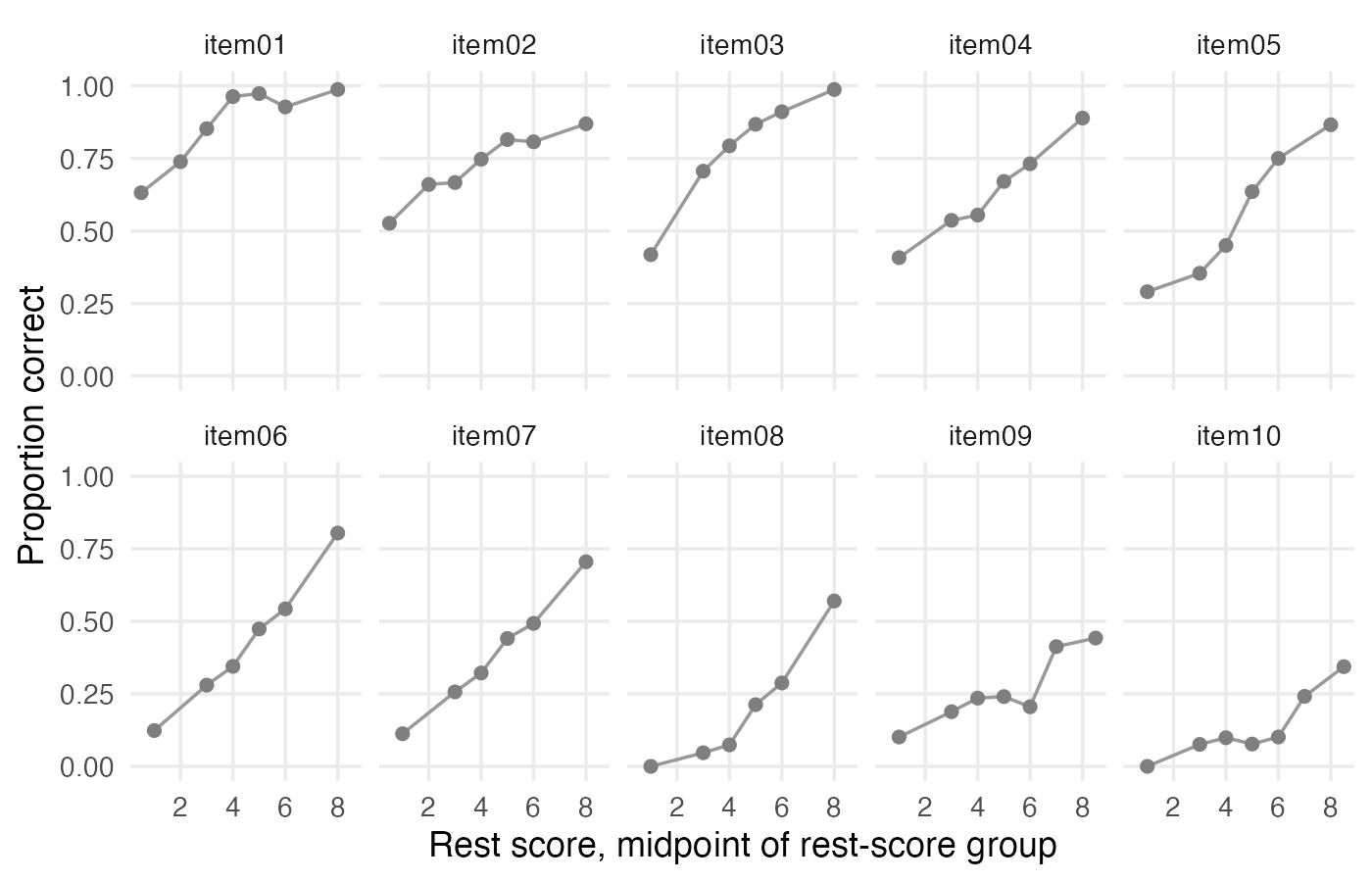
MSA was applied to the dichotomous scores of 500 fifth-grade students on the 10 fraction items. There were no missing data. Proportions correct ranged from .13 for Item 10 to .88 for Item 1, and the total score had a mean of 4.97 ($SD$ = 2.26). To check the data against the MHM, the item-pair coefficients and the rest-score regressions were examined. None of the 45 $H_{ij}$ was negative, and the smallest was .11. The monotonicity check detected no significant violation and no value of the crit statistic above 80, and the largest value was 18 (Figure 2).
To evaluate the items and the scale against the prespecified criterion of .30, $H_i$ and $H$ were estimated with standard errors and Wald 95% confidence intervals (Table 1). Three of the 10 items had $H_i$ below .30 (Figure 1). These were Item 2 ($H_i$ = .227, $SE$ = 0.042), Item 4 ($H_i$ = .279, $SE$ = 0.036), and Item 9 ($H_i$ = .223, $SE$ = 0.042), with proportions correct of .74, .62, and .25. The other seven items had $H_i$ from .323 to .455. The scale coefficient was $H$ = .337 ($SE$ = 0.023, 95% $CI$ = [.293, .382]).
Table 1. Scalability coefficients of the 10 items and the scale
| Item | H | SE | 95% CI lower | 95% CI upper |
|---|---|---|---|---|
| Item 1 | 0.455 | 0.052 | 0.354 | 0.557 |
| Item 2 | 0.227 | 0.042 | 0.144 | 0.311 |
| Item 3 | 0.429 | 0.034 | 0.363 | 0.495 |
| Item 4 | 0.279 | 0.036 | 0.209 | 0.349 |
| Item 5 | 0.338 | 0.032 | 0.274 | 0.401 |
| Item 6 | 0.360 | 0.032 | 0.298 | 0.422 |
| Item 7 | 0.323 | 0.033 | 0.259 | 0.388 |
| Item 8 | 0.452 | 0.031 | 0.391 | 0.513 |
| Item 9 | 0.223 | 0.042 | 0.140 | 0.306 |
| Item 10 | 0.381 | 0.052 | 0.279 | 0.483 |
| Scale | 0.337 | 0.023 | 0.293 | 0.382 |
Figure 1. Item scalability coefficients with 95% confidence intervals and a reference line at 0.30
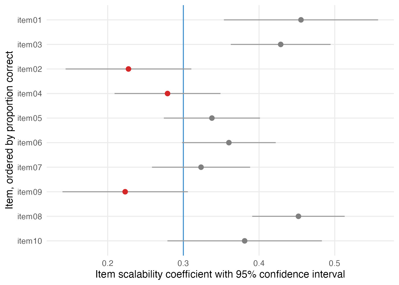
Figure 2. Proportion correct by rest-score group for each item
Discussion
MSA was used to examine whether the total score on the 10-item fraction test orders fifth-grade students by fraction understanding, and three of the 10 items had scalability coefficients below 0.30. Following the prespecified criterion, the 10-item total score was not used to rank students for small-group instruction.
The coefficients of Items 2, 4, and 9 indicate that responses to these items were weakly associated with responses to the other nine items, relative to the largest association that the proportions correct allow. The three items had proportions correct of 0.74, 0.62, and 0.25, so the low coefficients were not confined to easy or hard items. The other seven items met the criterion, and the scale coefficient of 0.337 falls in the range that Mokken (1971) labels weak. In a weak scale, the total score orders students with low precision, which matters most for students close to the selection cutoff. Ranking students by total score requires revising Items 2, 4, and 9 and estimating the coefficients in a new administration.
Limitations
This conclusion rests on local independence. Items that share solution steps add covariance that $\theta$ does not account for. Each affected $H_{ij}$ then rises by the added covariance divided by its $\mathrm{Cov_{\max}}$, and $H_i$ and $H$ rise with it. The coefficients describe the 500 students in the district schools that agreed to take part and do not extend to fifth-grade students in schools that did not take part.